Study Session 3 - Reading 9 Common Probability Distributions

LOS 9a: Explain a probability distribution and distinguish between discrete and continous random variables

• A probability distribution is the probabilities of all possible outcomes for a random variable.
• Discrete random variables are finite and countable (e.g. number of days on which it rained) whereas a continuous random variable can be an infinite number (e.g. rainfall for each day - the possible outcomes between 1 and 2 inches is infinite 1.00001, 1.0002, etc.) and is described as ranges instead (e.g. prob. that rainfall will be between 1 and 2 inches or, say, less than 1 inch).

LOS 9b: Describe the set of possible outcomes of a specified discrete random variable

• For discrete distribution p(x)=0 when it cannot occur and p(x) > 0 when it can.
• p(x) means the prob that rand. variable X=x
• For continous distribution p(x)=0 even though x can occur (because x cannot be a single value) so only p(x1 <>
• For price changes, generally use continuos e.g. prob. that price will be between $1 and $2
  

LOS 9c: Interpret a probability function, a probability density function, and a cumulative distribution function

• Probability function p(x) is the prob. that a rand. variable = a specific value.
• Two key properties:
  • 0 ≤ p(x)≤ 1
  • Sum of p(x) = 1 ... this makes sense since the sum of all probabilities should be 1
• Both the PDF and the CDF are cumulative functions
• A probability density function (or pdf) describes a probability function in the case of a continuous random variable. Also known as simply the “density”, a probability density function is denoted by “f(x)”. Since a pdf refers to a continuous random variable, its probabilities would be expressed as ranges of variables rather than probabilities assigned to individual values as is done for a discrete variable. For example, if a stock has a 20% chance of a negative return, the pdf in its simplest terms could be expressed as:
• A cumulative distribution function (cdf) is constructed by summing up, or cumulating all values in the probability function that are less than or equal to x and is very similar to the cum. freq. except for probabilities. May be expressed as F(x) = P(x ≤ x)

LOS 9d: Calculate and interpret probabilities for a random variable, given its cumulative distribution function
Take a prob. function for X={1,2,3,4], p(x) = x/10 which means that for the set of the whole numbers 1,2,3,4 the probability of each is 10%, therefore, f(3) is 0.6 which is the sum of 1/10, 2/10 and 3/10 i.e. the cumulative probabilities of all numbers up to and including the number in question. Same process if the prob's are different for each outcome.

LOS 9e: Define a discrete uniform random variable and a binomial random variable

• The above function is a discrete uniform random variable i.e. the prob. of each number occuring is equal i.e. for x={a,b,c] the p(a)=p(b)=p(c)
• The prob. for a range of outcomes is p(x)k where k is the number of possible outcomes in a range
• binomial random variable is the number of "successes" given a number of trials where the outcome is binary ("success" or "failure"). Might be used for the probability of a stock moving up once to $4.55 (the "success" is the up move might be duu where the d and u cancel) after n periods (the number of trials).
• Definition of "success" is crucial to this working out.

LOS 9f: Calculate and interpret probabilities given the discrete uniform and the binomial distribution functions

In English, this says multiply the number of combinations that you could have x successes out of n trials by the proportionate prob of success and by the proportionate prob of failure.

Expected value of X for Binomial Random Variable
For a given series of n trials, the expected value is n * p
i.e. if we perform n trials and the prob. of success on each trial is p we expect np successes.

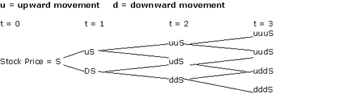
LOS 9g: Construct a binomial tree to describe stock price movement
this is fairly straightforward. Remember: If the up movement is 1.05 it means the price increases by 5% so mult. 1.05 by the stock price. the down movement will be the reciprocal 1/1.05.

LOS 9h: Describe the continuous uniform distribution and calculate and interpret probabilities, given a continuous uniform probability distribution

• A continuous uniform distribution describes a range of outcomes, usually bound with an upper and lower limit (say a and b), where any point in the range is a possibility.
• Since it is a range, there are infinite possibilities within the range. In addition, all outcomes are all equally likely (i.e. they are spread uniformly throughout the range).
• To calculate probabilities, find the area under a pdf curve.
• Basically, take the range between a and b is 100% of the prob. so the 100 divided by all the values between a and b gives you the prob. for each. Sum the number of values in the range you are looking for and mult. them by the prob. of each.
• Technically, this is achieved by the following: P(x1 ≤ X ≤ x2) = (x2-x1)/(b-a) where x1 to x2 is the value range you are looking for and b to a is the range of all values.

LOS 9i: Explain the key properties of the normal distribution, distinguish between a univariate and a multivariate distribution, and explain the role of correlation in the multivariate normal distribution

Normal distribution has following properties:

• completely described by mean and variance
• skewness = 0 and kurtosis = 3
• the tails are asymptotic
• 90% = 1.65
• 95% = 1.96
• 99% = 2.58

Univariate = distribution of one variable

Multivariate distribution

• is dist. of more than one variable and is meangingful only when the variables are dependent on one another.
• If the return of each variable is normally dist. then the distribution of the portfolio will be normal as well.
• Want a low correlation among your portfolio assets.
• 0.5n(n-1) will tell you the number of variances and means you need to describe mult. distribution

LOS 9j: Determine the probability that a normally distributed random variable lies inside a given confidence interval
if μ is $1 and σ is 5% we can say that 66% of the time, the expected return will be ± 5% (one σ) or between $0.95 and $1.05. So the confidence intervals for this example will be:

• 66% = x±1σ
• 90% = x±1.65σ
• 95% = x±1.97σ
• 90% = x±2.58σ

LOS 9k: Define the standard normal distribution, explain how to standardise a random variable, and calculate and interpret probabilities using the standard normal distribution

Standardise translates the value into a number of standard deviations so it can be compared to confidence intervals and a probability determined. This is called the z-value and is the diff. between the observation and the mean divided by the standard deviation or:

A z value of +1 would mean that the obs is one standard deviation above the mean, a z value of -1 means it falls one standard deviation below the mean.

Calculating Prob's using z-values
Standardise the value and then look up the appropriate prob. in the z-table.

• NB watch out for greater than or less than since the z-table is cumulative.
• If your z-value is 1.65 and you want to know prob of outcome being less than x then prob. is 90% since 90% of outcomes fall below x.
• If you want to know prob of outcome being more than x then prob is 1-0.90 or 10% because this is the small bit that isn't covered in the 90%

LOS 9l: Define shortfall risk, calculate the safety first ratio, and select an optimal portfolio using Roy's safety first criterion

• Shortfall risk is focus on both risk and return as opposed to simply the return
• 
• Maximise SFR i.e. just like with Sharpe ratios, you want the highest SFR possible as it gives you the best prob. of returns greater than threshold.

LOS 9m: Explain the relationship between normal and lognormal distributions and why the lognormal distribution is used to model asset prices

• Normal dist. are bilaterally symmetric and can take on any value
• lognormal is always greater than zero and skews to the right
• lognormal is generated by e^x and natural log (ln) of e^x is x
• lognormal for asset prices because they cannot be negative
• lognormal for modeling price relatives i.e. end of period divided by begin price

LOS 9n: Distinguish between discretely and continuously compounded rates of return and interpret a continuously compounded rate of return, given a specific holding period

• use discrete (normal) compounding for interest that compounds during specific times
• use continuous (lognormal) compounding for continous
• Annual rate (continuous) is ln(1+HPR) or rate of return[2nd][e^x]-1 e.g. if portfolio returned 20% then continuous compounding is found by ln 1.20
• Get return from annual rate (or holding period return) by reversing it i.e. 1+annual rate [ln]

LOS 9o: Explain Monte Carlo simulation and historical simulation and describe their major applications and limitations

Monte Carlo

• allows for "what if?"
• can simulate many possible variables and situations
• complex but is only as good as the underlying assumptions

Historical simulation

• based on historical data but past performance does not guarantee future results
• does not allow "what if?" scenarios